A distribution with an inverse cumulative distribution function (CDF) can be sampled from using just samples from \(U[0, 1]\). The inverse CDF (sometimes called the quantile function) is the value of \(x\) such that \(F_X(x) = Pr(X \leq x) = p\). Consider a that a transformation \(g: [0, 1] \rightarrow \mathbb{R}\), exists which takes a value sampled from the standard uniform distribution \(u \sim U[0, 1]\) and returns a value distributed according to the target distribution. Then the inverse CDF can be written as:
Since the CDF of the uniform distribution over the interval \([0, 1]\) is:
$$\[\begin{align*}
F_U(u) =
\begin{cases}
0 & u < 0 \\
u & u \in [0, 1) \\
1 & u \geq 1
\end{cases}
\end{align*}\]$$
Then \(F_x^{-1}(X) = g(x)\) as required. The algorithm below summarises the inverse sampling procedure.
Sample \(u \sim U[0, 1]\)
Evaluate \(x = F^{-1}(u)\)
Return \(x\)
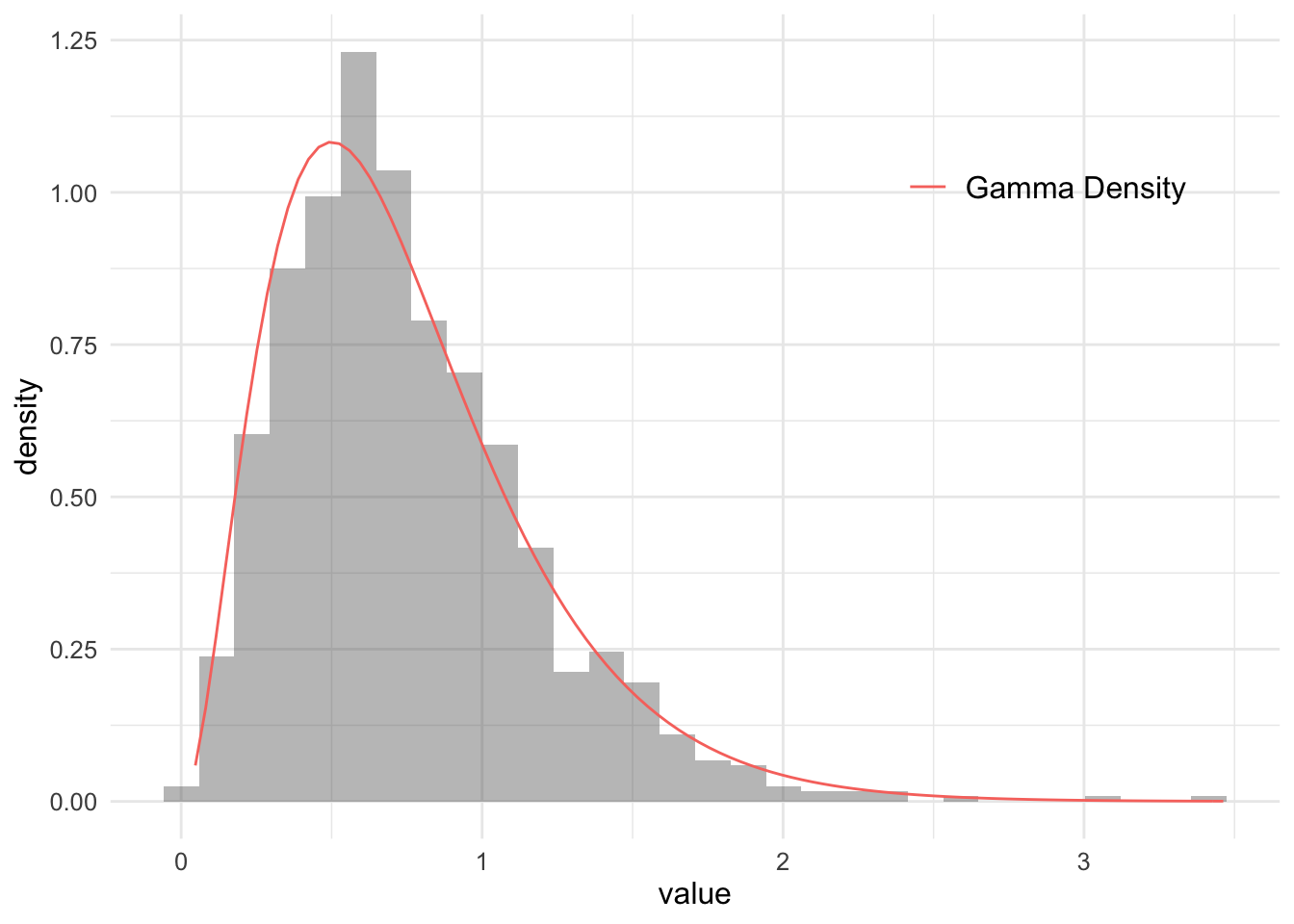
Most statistical packages will expose the quantile function for common distributions making it practical to use inverse sampling. The figure below shows a histogram of 1,000 simulated values from a \(\textrm{Gamma}(3, 4)\) distribution using the inverse CDF method, the analytical density is plotted in red.
The figure below shows samples from \(\textrm{Gamma}(3, 4)\) using the inverse CDF method plotted with the analytical PDF.